Lab Notebook Entry #20

Steel current collectors for all-Fe, first Cu/Mn static cell test
lab notebook
research
flow batteries
doi
Author

Kirk Pollard Smith

Published

September 26, 2026

Did another test with all-iron, but with a carbon steel current collector, and a first static cell test of Cu/Mn system (based on Daniel’s tests here), both not very great tests but working out bugs and moving ahead.

Cu/Mn test

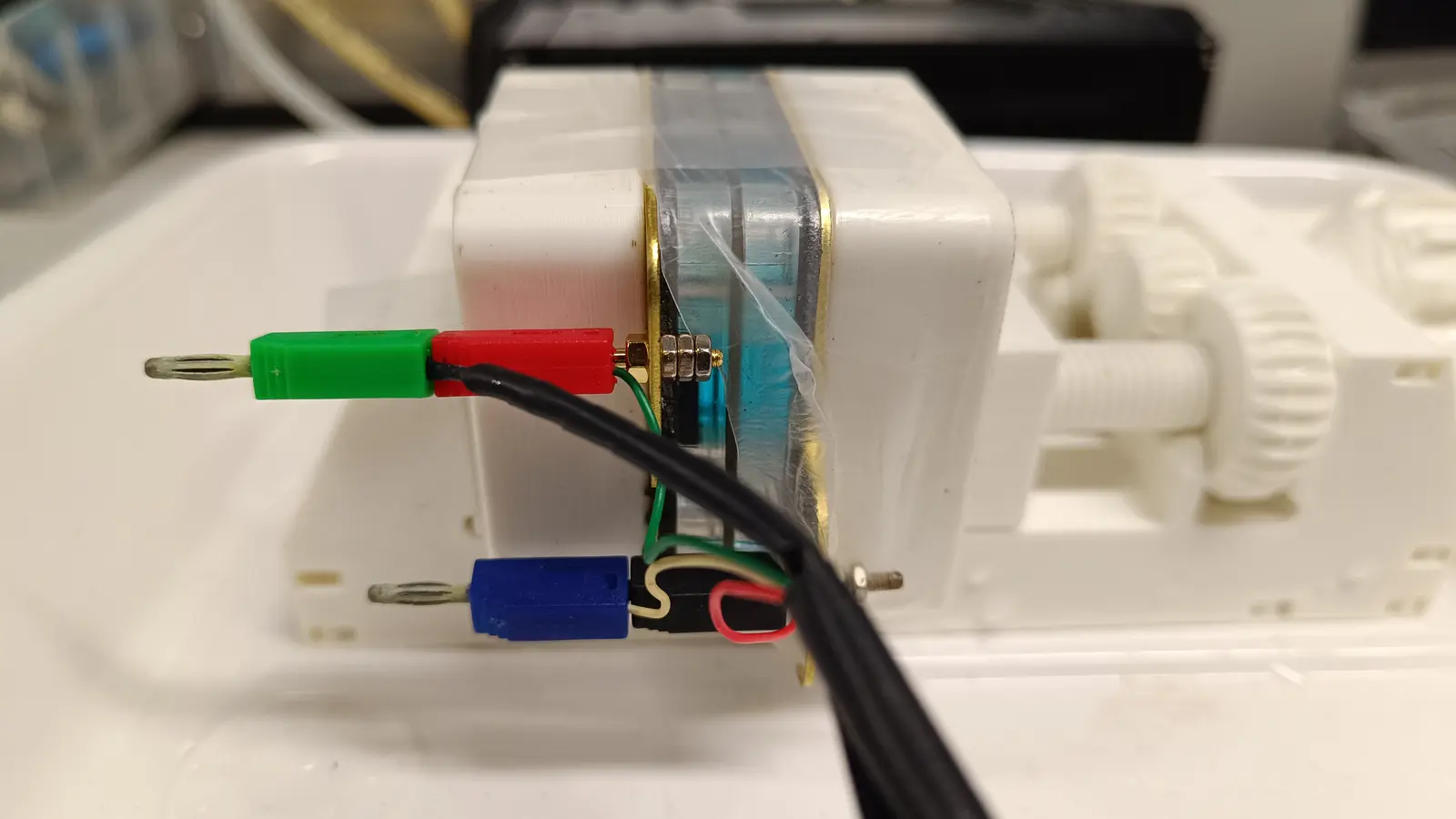
The Cu/Mn cell, which is just one of our flow cells but sealed and filled from the top with a syringe.

Here is the raw data for Cu/Mn.

Electrolyte Composition (molarity, per L solution) Unreported, lack of good volume measurement
Electrolyte Composition (molality, per kg solution) 0.54 m CuSO4, 0.52 m MnSO4, 0.00 m FeSO4, 2.01 m MSA, 32.38 m H2O
Electrolyte Volume Equivalent of of 3.6 g of electrolyte
Electrolyte Density Unreported, likely around 1.2 g/mL
Cell Geometric Area 2 cm2
Separator None
Anode Configuration Grafoil + 3.2 mm graphite felt placed on top, no compression mechanism
Cathode Configuration Copper foil over grafoil
Gaskets Outer and inner, 0.40 mm silicone (measured with micrometer)
Current Density 10 mA/cm2
Charging Conditions To 1.25 V
Discharging Conditions To 0 V
Code
import pandas as pd
from tqdm import tqdm, notebook
import numpy as np
import scipy
import plotly.express as px
import plotly.graph_objects as go
from plotly.subplots import make_subplots
import kaleido
from IPython.display import Image

tqdm_disabled = True  # True for website, change to False for local work
electrolyte = "Cu/Mn"

sampling = True

MIN_POINTS0 = 500
DIFF_LIMIT = 0.1

VOLUME_TO_RESERVOIRS = 3 # unrecorded this time - electrolyte volume in mL, approx, measured by syring when adding to reservoirs
MASS_TO_RESERVOIRS =  3.60 # g of electrolyte actually loaded into system, based on weighing syringe before/after loading reservoirs

density = MASS_TO_RESERVOIRS / VOLUME_TO_RESERVOIRS

# molecular weights in g/mol

# electrolyte component masses, in g

###    Cu/Mn    ###

MASS_CuSO4        = 2.00 # PENTAHYDRATE
MASS_MnSO4        = 1.29 # MONOHYDRATE
MASS_MSA_99pct    = 2.88 # >99.0% w/w solution
MASS_FeSO4        = 0.00 # HEPTAHYDRATE - forgot to add it, should be 0.1 g
MASS_H2O          = 7 + 1.57 # 1.5 mL more than Daniel said to get all dissolved

total_mass_kg = (MASS_CuSO4 + MASS_MnSO4 + MASS_MSA_99pct + MASS_FeSO4 + MASS_H2O) / 1000.0

MW_CuSO4        = 249.685 # PENTAHYDRATE
MW_MnSO4        = 169.02  # MONOHYDRATE
MW_MSA          = 96.10
MW_FeSO4        = 278.02  # HEPTAHYDRATE
MW_H2O          = 18.01528

molality_CuSO4          = MASS_CuSO4 / MW_CuSO4 / total_mass_kg
molality_MnSO4          = MASS_MnSO4 / MW_MnSO4 / total_mass_kg
molality_FeSO4          = MASS_FeSO4 / MW_FeSO4 / total_mass_kg
molality_MSA            = MASS_MSA_99pct*0.99 / MW_MSA / total_mass_kg
molality_H2O            = (MASS_H2O + 0.01*MASS_MSA_99pct) / MW_H2O / total_mass_kg

molarity_CuSO4 = MASS_CuSO4 / MW_CuSO4 / (total_mass_kg/density)
molarity_MnSO4 = MASS_MnSO4 / MW_MnSO4 / (total_mass_kg/density)
molarity_FeSO4 = MASS_FeSO4 / MW_FeSO4 / (total_mass_kg/density)
molarity_MSA = MASS_MSA_99pct*0.99 / MW_MSA / (total_mass_kg/density)
molarity_H2O = (MASS_H2O + 0.01*MASS_MSA_99pct) / MW_H2O / (total_mass_kg/density)

###   ALL-IRON  ###

# MASS_FeCl2_2H2O   = 1.60
# MASS_MgCl2        = 4.30
# MASS_AscorbicAcid = 0.06 # wasn't able to properly record it
# MASS_HCl_15pct    = 0.06 # 15% w/w solution
# MASS_H2O          = 9.49

# total_mass_kg = (MASS_FeCl2_2H2O + MASS_MgCl2 + MASS_AscorbicAcid + MASS_HCl_15pct + MASS_H2O) / 1000.0

# MW_FeCl2_2H2O   = 162.78
# MW_MgCl2        = 95.211
# MW_AscorbicAcid = 176.124
# MW_HCl          = 36.46
# MW_H2O          = 18.01528

# molality_FeCl2 = MASS_FeCl2_2H2O / MW_FeCl2_2H2O / total_mass_kg
# molality_MgCl2 = MASS_MgCl2 / MW_MgCl2 / total_mass_kg
# molality_AscorbicAcid = MASS_AscorbicAcid / MW_AscorbicAcid / total_mass_kg
# molality_HCl = MASS_HCl_15pct*0.15 / MW_HCl / total_mass_kg
# molality_H2O = (MASS_H2O + 0.85*MASS_HCl_15pct) / MW_H2O / total_mass_kg

# molarity_FeCl2 = MASS_FeCl2_2H2O / MW_FeCl2_2H2O / VOLUME_TO_RESERVOIRS * 1000.0
# molarity_MgCl2 = MASS_MgCl2 / MW_MgCl2 / VOLUME_TO_RESERVOIRS * 1000.0
# molarity_AscorbicAcid = MASS_AscorbicAcid / MW_AscorbicAcid / VOLUME_TO_RESERVOIRS * 1000.0
# molarity_HCl = MASS_HCl_15pct*0.15 / MW_HCl / VOLUME_TO_RESERVOIRS * 1000.0
# molarity_H2O = (MASS_H2O + 0.85*MASS_HCl_15pct) / MW_H2O / VOLUME_TO_RESERVOIRS * 1000.0


### ZINC-IODIDE ###

# MASS_ZnCl2  = 1.37
# MASS_NH4Cl  = 1.06
# MASS_KI     = 3.31
# MASS_H2O    = 8.52
# MASS_TriEG  = 0.63

# total_mass_kg = (MASS_ZnCl2 + MASS_KI + MASS_H2O + MASS_TriEG) / 1000.0

# MW_ZnCl2 = 136.315
# MW_NH4Cl = 53.49
# MW_KI = 166.0028
# MW_H2O = 18.01528
# MW_TriEG = 150.174

# molality_ZnCl2 = MASS_ZnCl2 / MW_ZnCl2 / total_mass_kg
# molality_NH4Cl = MASS_NH4Cl / MW_NH4Cl / total_mass_kg
# molality_KI = MASS_KI / MW_KI / total_mass_kg
# molality_TriEG = MASS_TriEG / MW_TriEG / total_mass_kg
# molality_H2O = MASS_H2O / MW_H2O / total_mass_kg

# molarity_ZnCl2 = MASS_ZnCl2 / MW_ZnCl2 / VOLUME_TO_RESERVOIRS * 1000.0
# molarity_NH4Cl = MASS_NH4Cl / MW_NH4Cl / VOLUME_TO_RESERVOIRS * 1000.0
# molarity_KI = MASS_KI / MW_KI / VOLUME_TO_RESERVOIRS * 1000.0
# molarity_TriEG = MASS_TriEG / MW_TriEG / VOLUME_TO_RESERVOIRS * 1000.0
# molarity_H2O = MASS_H2O / MW_H2O / VOLUME_TO_RESERVOIRS * 1000.0


filenames = [
    "03-06-2026-KPS-28.zip",
]


all_data = []
for f in filenames:
    if len(all_data) == 0:
        all_data.append(pd.read_csv(f, delimiter="\t").dropna())
    else:
        df0 = pd.read_csv(f, delimiter="\t").dropna()
        df0["Elapsed time(s)"] += all_data[-1]["Elapsed time(s)"].iat[-1]
        all_data.append(df0)


df = pd.concat(all_data, ignore_index=True)

if not tqdm_disabled:
    print("Electrolyte Composition:")
    if electrolyte=="zinc":
        print(
            "Molarities (moles/L solution): {:.2f} M ZnCl~2~, {:.2f} M NH~4~Cl, {:.2f} M KI, {:.2f} M triethylene glycol, {:.2f} M H~2~O\n".format(
                molarity_ZnCl2, molarity_NH4Cl, molarity_KI, molarity_TriEG, molarity_H2O
            )
        )
        print(
            "Molalities (moles/kg solution): {:.2f} m ZnCl~2~, {:.2f} m NH~4~Cl, {:.2f} m KI, {:.2f} m triethylene glycol, {:.2f} m H~2~O\n".format(
                molality_ZnCl2, molality_NH4Cl, molality_KI, molality_TriEG, molality_H2O
            )
        )
    elif electrolyte=="iron":
        print(
            "Molarities (moles/L solution): {:.2f} M FeCl~2~, {:.2f} M MgCl~2~, {:.2f} M ascorbic acid, {:.2f} M HCl, {:.2f} M H~2~O\n".format(
                molarity_FeCl2, molarity_MgCl2, molarity_AscorbicAcid, molarity_HCl, molarity_H2O
            )
        )
        print(
            "Molalities (moles/kg solution): {:.2f} m FeCl~2~, {:.2f} m MgCl~2~, {:.2f} m ascorbic acid, {:.2f} m HCl, {:.2f} m H~2~O\n".format(
                molality_FeCl2, molarity_MgCl2, molarity_AscorbicAcid, molarity_HCl, molarity_H2O
            )
        )
    elif electrolyte=="Cu/Mn":
        print(
            "Molarities (moles/L solution): {:.2f} M CuSO~4~, {:.2f} M MnSO~4~, {:.2f} M FeSO~4~, {:.2f} M MSA, {:.2f} M H~2~O\n".format(
                molarity_CuSO4, molarity_MnSO4, molarity_FeSO4, molarity_MSA, molarity_H2O
            )
        )
        print(
            "Molalities (moles/kg solution): {:.2f} m CuSO~4~, {:.2f} m MnSO~4~, {:.2f} m FeSO~4~, {:.2f} m MSA, {:.2f} m H~2~O\n".format(
                molality_CuSO4, molality_MnSO4, molality_FeSO4, molality_MSA, molality_H2O
            )
        )

    else:
        print("WARNING: Specify the type of electrolyte")
        
    print("Density approx. {:.1f} g/mL\n".format(density))
    print(
        "Experiment length: {:.1f} hours".format(
            all_data[-1]["Elapsed time(s)"].iat[-1] / 3600.0
        )
    )

df["mean_current"] = df["Current(A)"].rolling(4).mean()
df["prev_current"] = df["mean_current"].shift(-1)
df["VChange"] = df["Potential(V)"].diff().abs()
df["is_OCP"] = (abs(df["mean_current"])<0.0001).astype(int)
df["is_change"] = (
    (((df["mean_current"] > 0) & (df["prev_current"] < 0))
    | ((df["mean_current"] < 0) & (df["prev_current"] > 0)))
    #& df["is_OCP"]==False #current must be greater than 0.5 mA to avoid OCP holds
).astype(int)
df["is_start_charge"] = ((df["prev_current"] < -0.001) & (df["is_OCP"]== 1)).astype(int)
df["is_start_discharge"] = ((df["prev_current"] > 0.001) & (df["is_OCP"]== 1)).astype(int)


idx_changes = list(df[(df["is_start_charge"] == 1) | (df["is_start_discharge"] == 1)].index)
idx_changes.append(len(df) - 1)
all_curves = []
idx_start = 0
for idx in tqdm(idx_changes, disable=tqdm_disabled):
    if len(df.iloc[idx_start:idx, :]) > 50:
        all_curves.append(df.iloc[idx_start:idx, :])
    idx_start = idx


results = []
n_curves = np.max([1, int(np.floor(len(all_curves) / 2))])
n_curves = 18

for CN in notebook.tnrange(n_curves, disable=tqdm_disabled):
    CURVE_N1 = CN * 2
    CURVE_N2 = CN * 2 + 1

    # Process charge data

    if sampling:
        N_TERM_POINTS = int(np.min([MIN_POINTS0, len(all_curves[CURVE_N1]) / 2.0]))
        MIN_POINTS = int(
            np.min([MIN_POINTS0, len(all_curves[CURVE_N1]) - N_TERM_POINTS * 2])
        )

        df0 = pd.concat(
            [
                all_curves[CURVE_N1].iloc[:N_TERM_POINTS],
                all_curves[CURVE_N1]
                .iloc[N_TERM_POINTS:-N_TERM_POINTS]
                .sample(n=MIN_POINTS),
                all_curves[CURVE_N1].iloc[-N_TERM_POINTS:],
            ]
        ).sort_values("Elapsed time(s)", ascending=True)
        df0 = df0[df0["VChange"] < DIFF_LIMIT]
    else:
        df0 = all_curves[CURVE_N1].copy()
    df0["mAh"] = np.abs(
        scipy.integrate.cumulative_trapezoid(
            df0["Current(A)"], df0["Elapsed time(s)"], initial=0
        )
        * 1000.0
        / 3600.0
    )
    total_energy0 = scipy.integrate.cumulative_trapezoid(
        df0["Current(A)"].abs() * df0["Potential(V)"],
        df0["Elapsed time(s)"],
        initial=0.0,
    )[-1]

    # Process discharge data
    if sampling:
        N_TERM_POINTS = int(np.min([MIN_POINTS0, len(all_curves[CURVE_N2]) / 2.0]))
        MIN_POINTS = int(
            np.min([MIN_POINTS0, len(all_curves[CURVE_N2]) - N_TERM_POINTS * 2])
        )
        df1 = pd.concat(
            [
                all_curves[CURVE_N2].iloc[:N_TERM_POINTS],
                all_curves[CURVE_N2]
                .iloc[N_TERM_POINTS:-N_TERM_POINTS]
                .sample(n=MIN_POINTS),
                all_curves[CURVE_N2].iloc[-N_TERM_POINTS:],
            ]
        ).sort_values("Elapsed time(s)", ascending=True)
        df1 = df1[df1["VChange"] < DIFF_LIMIT]
    else:
        df1 = all_curves[CURVE_N2].copy()

    df1["mAh"] = np.abs(
        scipy.integrate.cumulative_trapezoid(
            df1["Current(A)"], df1["Elapsed time(s)"], initial=0.0
        )
        * 1000.0
        / 3600.0
    )
    total_energy1 = scipy.integrate.cumulative_trapezoid(
        df1["Current(A)"].abs() * df1["Potential(V)"],
        df1["Elapsed time(s)"],
        initial=0.0,
    )[-1]

    CE = 100.0 * (df1["mAh"].iloc[-1] / df0["mAh"].iloc[-1])
    EE = 100.0 * (total_energy1 / total_energy0)
    VE = 100.0 * EE / CE
    results.append(
        {
            "Number": CN + 1,
            "CE": CE,
            "VE": VE,
            "EE": EE,
            "Charge_potential": df0["Potential(V)"].mean(),
            "Discharge_potential": df1["Potential(V)"].mean(),
            "Charge_stored": df1["mAh"].iloc[-1] / VOLUME_TO_RESERVOIRS,
            "Energy_density_discharge": total_energy1 / VOLUME_TO_RESERVOIRS / 3600.0 * 1000,
        }
    )

    # Save the modified DataFrames back to the all_curves list
    all_curves[CURVE_N1] = df0
    all_curves[CURVE_N2] = df1

results_df = pd.DataFrame(results)

if not tqdm_disabled:
    print(results_df)
    print("")
    print(results_df.mean())
Code
# Color gradient for charge curves
charge_colors = [
    px.colors.sequential.Blues[int(i)]
    for i in np.linspace(3, len(px.colors.sequential.Blues) - 1, n_curves)
]
discharge_colors = [
    px.colors.sequential.Greys[int(i)]
    for i in np.linspace(3, len(px.colors.sequential.Greys) - 1, n_curves)
]


# Plot charge/discharge curves
fig1 = go.Figure()
for CN in range(n_curves):

    CURVE_N1 = CN * 2
    CURVE_N2 = CN * 2 + 1
    fig1.add_trace(
        go.Scatter(
            x=all_curves[CURVE_N1]["mAh"] / VOLUME_TO_RESERVOIRS,
            y=all_curves[CURVE_N1]["Potential(V)"],
            mode="lines",
            name=f"Charge {CN+1}",
            line=dict(color=charge_colors[CN], dash="solid"),
            showlegend=False,
        )
    )
    fig1.add_trace(
        go.Scatter(
            x=all_curves[CURVE_N2]["mAh"] / VOLUME_TO_RESERVOIRS,
            y=all_curves[CURVE_N2]["Potential(V)"],
            mode="lines",
            name=f"Discharge {CN+1}",
            line=dict(color=discharge_colors[CN], dash="solid"),
            showlegend=False,
        )
    )
fig1.update_layout(
    xaxis_title="Capacity (Ah/L)",
    yaxis_title="Potential (V)",
    legend=dict(orientation="h", yanchor="bottom", y=0.02, xanchor="right", x=0.99),
    hoverlabel=dict(
        bgcolor="white",
    ),
    xaxis=dict(range=[-1, 5]),
    yaxis=dict(range=[-.49, 1.5]),


)

fig1.add_trace(
    go.Scatter(
        x=[None],
        y=[None],
        mode="lines",
        line=dict(color=charge_colors[0], dash="solid"),
        name="Charge (cycle 1)",
    )
)
fig1.add_trace(
    go.Scatter(
        x=[None],
        y=[None],
        mode="lines",
        line=dict(color=charge_colors[-1], dash="solid"),
        name=f"Charge (cycle {n_curves})",
    )
)
fig1.add_trace(
    go.Scatter(
        x=[None],
        y=[None],
        mode="lines",
        line=dict(color=discharge_colors[0], dash="solid"),
        name="Discharge (cycle 1)",
    )
)
fig1.add_trace(
    go.Scatter(
        x=[None],
        y=[None],
        mode="lines",
        line=dict(color=discharge_colors[-1], dash="solid"),
        name=f"Discharge (cycle {n_curves})",
    )
)

fig1.show()
Code
# Plot efficiency
fig2 = px.scatter(
    results_df,
    x="Number",
    y=["VE", "CE", "EE"],
    labels={"value": "Efficiency (%)", "variable": "Metric"},
)
fig2.update_traces(mode="markers")


fig2.update_layout(
    yaxis=dict(range=[-10, 100]),
    legend=dict(
        orientation="v",
        yanchor="bottom",
        y=0.02,
        xanchor="right",
        x=0.99
    )
)


fig2.show()

Charge/discharge efficiencies

Code
fig5 = px.scatter(
    results_df,
    x="Number",
    y="Energy_density_discharge",
    labels={
        "Energy_density_discharge": "Energy Density on Discharge (Wh/L)",
        "Number": "Cycle Number",
    },
    range_y=[0,1.2*max(results_df["Energy_density_discharge"])]
)

max_val = results_df["Energy_density_discharge"].max()
mean_val = results_df["Energy_density_discharge"].mean()

fig5.add_hline(y=max_val, line_dash="dash", line_color="black", annotation_text="Max", annotation_position="top right",annotation_font_size = 10)
fig5.add_hline(y=mean_val, line_dash="dash", line_color="blue", annotation_text="Mean", annotation_position="top right",annotation_font_size = 10)
fig5.add_hline(y=0.8*max_val, line_dash="dash", line_color="red", annotation_text="80% Max", annotation_position="top right",annotation_font_size = 10)

fig5.show()

Discharge energy densities

Code
norm_charge = results_df["Charge_potential"] / results_df["Charge_potential"].iloc[0]
norm_discharge = results_df["Discharge_potential"] / results_df["Discharge_potential"].iloc[0]

fig6 = go.Figure()
fig6.add_trace(go.Scatter(
    x=results_df["Number"],
    y=norm_charge,
    mode="lines+markers",
    name="Charge Potential"
))
fig6.add_trace(go.Scatter(
    x=results_df["Number"],
    y=norm_discharge,
    mode="lines+markers",
    name="Discharge Potential"
))
fig6.update_layout(
    xaxis_title="Cycle Number",
    yaxis_title="Normalized Potential",
    legend=dict(
        orientation="v",
        yanchor="top",
        y=0.95,
        xanchor="left",
        x=0.05
    )
)

fig6.show()

Average charge and discharge potentials normalized to first cycle

Code
table_df = (
    results_df.describe().loc[["mean", "std"]]
    .round(decimals=1)
    .drop(columns=["Number", "Charge_potential", "Discharge_potential"])
    .rename(
        columns={
            "CE": "Coulombic Efficiency (%)",
            "EE": "Energy Efficiency (%)",
            "VE": "Voltaic Efficiency (%)",
            "Charge_stored": "Discharge Capacity (Ah/L)",
            "Energy_density_discharge": "Energy Density (Wh/L)",
        }
    )
)

# Bar chart of efficiencies with error bars
eff_cols = ["Coulombic Efficiency (%)", "Voltaic Efficiency (%)", "Energy Efficiency (%)"]
eff_labels = ["Coulombic", "Voltaic", "Energy"]

means = table_df.loc["mean", eff_cols].values
stds = table_df.loc["std", eff_cols].values
Code
fig6 = go.Figure()
fig6.add_trace(go.Bar(
    x=eff_labels,
    y=means,
    error_y=dict(type="data", array=stds, visible=True),
    name="Efficiency",
    marker_color=["#1f77b4", "#ff7f0e", "#2ca02c"]
))
fig6.update_layout(
    yaxis_title="Efficiency (%)",
    yaxis=dict(range=[0, 100])
)
fig6.show()

Mean efficiency values with standard deviation

Code
cap_cols = ["Discharge Capacity (Ah/L)"]
cap_labels = ["Discharge Capacity"]

cap_means = table_df.loc["mean", cap_cols].values
cap_stds = table_df.loc["std", cap_cols].values

ed_cols = ["Energy Density (Wh/L)"]
ed_labels = ["Energy Density"]

ed_means = table_df.loc["mean", ed_cols].values
ed_stds = table_df.loc["std", ed_cols].values

fig_combined = make_subplots(rows=1, cols=2)

fig_combined.add_trace(
    go.Bar(
        x=cap_labels,
        y=cap_means,
        error_y=dict(type="data", array=cap_stds, visible=True),
        name="Capacity",
        marker_color="#1f77b4"
    ),
    row=1, col=1
)

fig_combined.add_trace(
    go.Bar(
        x=ed_labels,
        y=ed_means,
        error_y=dict(type="data", array=ed_stds, visible=True),
        name="Energy Density",
        marker_color="#2ca02c"
    ),
    row=1, col=2
)
top = max(max(cap_means + cap_stds), max(ed_means + ed_stds))*1.1
fig_combined.update_layout(
    yaxis=dict(title="Discharge Capacity (Ah/L)"),
    yaxis2=dict(title="Energy Density (Wh/L)", anchor="x2", overlaying="y", side="left"),
    yaxis_range=[0, top],
    yaxis2_range=[0, top],
    showlegend=False
)
fig_combined.show()

Mean discharge capacity and energy density values with standard deviation

I didn’t add Fe(II) scavenger to this cell, so the results aren’t very representative, but at least I got a cell built and the data plotting workflow for Cu/Mn. Next cell will have Fe, and then I want to try a conductive adhesive for the graphite felt to the graphite foil on the manganese side (positive).

Iron RFB test

Here is the raw data for the iron test.

Electrolyte Composition (molarity, per L solution) 0.89 M FeCl2, 4.11 M MgCl2, 0.03 M ascorbic acid, 0.02 M HCl, 48.15 M H2O
Electrolyte Composition (molality, per kg solution) 0.63 m FeCl2, 4.11 m MgCl2, 0.03 m ascorbic acid, 0.02 m HCl, 48.15 m H2O
Electrolyte Volume 5.5 mL (anolyte) + 5.5 mL (catholyte)
Electrolyte Density 1.4 g/mL
RFB Dev Kit commit e655c88f06
Cell Geometric Area 2 cm2
Separator Daramic AA-900
Anode Configuration Grafoil + 3.2 mm graphite felt
Cathode Configuration Grafoil + 3.2 mm graphite felt
Gaskets Outer and inner, 0.40 mm silicone (measured with micrometer)
Current Density 20 mA/cm2
Charging Conditions To 44 mAh (about 4 Ah/L) or 1.35 V
Discharging Conditions To 0 V
Flow Conditions Kamoer KPK200 24 V brushless peristaltic pumps at 40% duty cycle (about 1500 rpm) with 3.2x6.4 mm Tygon Chemical (PTFE-lined BPT) tubing, double reservoirs with Luer Lock barbed fittings
Inert Gas Sparged electrolyte through septa with argon for 15 minutes prior to cycling with pumps on, septa slightly open to allow gas to escape, then attached septa firmly, removed gas tubing with septa attached and put parafilm over septa.
Code
import pandas as pd
from tqdm import tqdm, notebook
import numpy as np
import scipy
import plotly.express as px
import plotly.graph_objects as go
from plotly.subplots import make_subplots
import kaleido
from IPython.display import Image

tqdm_disabled = True  # True for website, change to False for local work
electrolyte = "iron"

sampling = True

MIN_POINTS0 = 500
DIFF_LIMIT = 0.1

VOLUME_TO_RESERVOIRS = 11  # electrolyte volume in mL, approx, measured by taking as much electrolyte as possible up into a 12 mL syringe

MASS_TO_RESERVOIRS = 14.93  # g of electrolyte actually loaded into system, based on weighing syringe before/after loading reservoirs

density = MASS_TO_RESERVOIRS / VOLUME_TO_RESERVOIRS

# molecular weights in g/mol

# electrolyte component masses, in g

###   ALL-IRON  ###

MASS_FeCl2_2H2O   = 1.60
MASS_MgCl2        = 4.30
MASS_AscorbicAcid = 0.06 # wasn't able to properly record it
MASS_HCl_15pct    = 0.06 # 15% w/w solution
MASS_H2O          = 9.49

total_mass_kg = (MASS_FeCl2_2H2O + MASS_MgCl2 + MASS_AscorbicAcid + MASS_HCl_15pct + MASS_H2O) / 1000.0

MW_FeCl2_2H2O   = 162.78
MW_MgCl2        = 95.211
MW_AscorbicAcid = 176.124
MW_HCl          = 36.46
MW_H2O          = 18.01528

molality_FeCl2 = MASS_FeCl2_2H2O / MW_FeCl2_2H2O / total_mass_kg
molality_MgCl2 = MASS_MgCl2 / MW_MgCl2 / total_mass_kg
molality_AscorbicAcid = MASS_AscorbicAcid / MW_AscorbicAcid / total_mass_kg
molality_HCl = MASS_HCl_15pct*0.15 / MW_HCl / total_mass_kg
molality_H2O = (MASS_H2O + 0.85*MASS_HCl_15pct) / MW_H2O / total_mass_kg

molarity_FeCl2 = MASS_FeCl2_2H2O / MW_FeCl2_2H2O / VOLUME_TO_RESERVOIRS * 1000.0
molarity_MgCl2 = MASS_MgCl2 / MW_MgCl2 / VOLUME_TO_RESERVOIRS * 1000.0
molarity_AscorbicAcid = MASS_AscorbicAcid / MW_AscorbicAcid / VOLUME_TO_RESERVOIRS * 1000.0
molarity_HCl = MASS_HCl_15pct*0.15 / MW_HCl / VOLUME_TO_RESERVOIRS * 1000.0
molarity_H2O = (MASS_H2O + 0.85*MASS_HCl_15pct) / MW_H2O / VOLUME_TO_RESERVOIRS * 1000.0


### ZINC-IODIDE ###

# MASS_ZnCl2  = 1.37
# MASS_NH4Cl  = 1.06
# MASS_KI     = 3.31
# MASS_H2O    = 8.52
# MASS_TriEG  = 0.63

# total_mass_kg = (MASS_ZnCl2 + MASS_KI + MASS_H2O + MASS_TriEG) / 1000.0

# MW_ZnCl2 = 136.315
# MW_NH4Cl = 53.49
# MW_KI = 166.0028
# MW_H2O = 18.01528
# MW_TriEG = 150.174

# molality_ZnCl2 = MASS_ZnCl2 / MW_ZnCl2 / total_mass_kg
# molality_NH4Cl = MASS_NH4Cl / MW_NH4Cl / total_mass_kg
# molality_KI = MASS_KI / MW_KI / total_mass_kg
# molality_TriEG = MASS_TriEG / MW_TriEG / total_mass_kg
# molality_H2O = MASS_H2O / MW_H2O / total_mass_kg

# molarity_ZnCl2 = MASS_ZnCl2 / MW_ZnCl2 / VOLUME_TO_RESERVOIRS * 1000.0
# molarity_NH4Cl = MASS_NH4Cl / MW_NH4Cl / VOLUME_TO_RESERVOIRS * 1000.0
# molarity_KI = MASS_KI / MW_KI / VOLUME_TO_RESERVOIRS * 1000.0
# molarity_TriEG = MASS_TriEG / MW_TriEG / VOLUME_TO_RESERVOIRS * 1000.0
# molarity_H2O = MASS_H2O / MW_H2O / VOLUME_TO_RESERVOIRS * 1000.0


filenames = [
    "03-06-2026-KPS-27.zip",
    # "03-06-2026-KPS-28.zip",

]


all_data = []
for f in filenames:
    if len(all_data) == 0:
        all_data.append(pd.read_csv(f, delimiter="\t").dropna())
    else:
        df0 = pd.read_csv(f, delimiter="\t").dropna()
        df0["Elapsed time(s)"] += all_data[-1]["Elapsed time(s)"].iat[-1]
        all_data.append(df0)


df = pd.concat(all_data, ignore_index=True)

if not tqdm_disabled:
    print("Electrolyte Composition:")
    if electrolyte=="zinc":
        print(
            "Molarities (moles/L solution): {:.2f} M ZnCl~2~, {:.2f} M NH~4~Cl, {:.2f} M KI, {:.2f} M triethylene glycol, {:.2f} M H~2~O\n".format(
                molarity_ZnCl2, molarity_NH4Cl, molarity_KI, molarity_TriEG, molarity_H2O
            )
        )
        print(
            "Molalities (moles/kg solution): {:.2f} m ZnCl~2~, {:.2f} m NH~4~Cl, {:.2f} m KI, {:.2f} m triethylene glycol, {:.2f} m H~2~O\n".format(
                molality_ZnCl2, molality_NH4Cl, molality_KI, molality_TriEG, molality_H2O
            )
        )
    elif electrolyte=="iron":
        print(
            "Molarities (moles/L solution): {:.2f} M FeCl~2~, {:.2f} M MgCl~2~, {:.2f} M ascorbic acid, {:.2f} M HCl, {:.2f} M H~2~O\n".format(
                molarity_FeCl2, molarity_MgCl2, molarity_AscorbicAcid, molarity_HCl, molarity_H2O
            )
        )
        print(
            "Molalities (moles/kg solution): {:.2f} m FeCl~2~, {:.2f} m MgCl~2~, {:.2f} m ascorbic acid, {:.2f} m HCl, {:.2f} m H~2~O\n".format(
                molality_FeCl2, molarity_MgCl2, molarity_AscorbicAcid, molarity_HCl, molarity_H2O
            )
        )
    else:
        print("WARNING: Specify the type of electrolyte")
        
    print("Density approx. {:.1f} g/mL\n".format(density))
    print(
        "Experiment length: {:.1f} hours".format(
            all_data[-1]["Elapsed time(s)"].iat[-1] / 3600.0
        )
    )

df["mean_current"] = df["Current(A)"].rolling(3).mean()
df["prev_current"] = df["mean_current"].shift(-1)
df["VChange"] = df["Potential(V)"].diff().abs()
df["is_OCP"] = (abs(df["mean_current"])<0.0001).astype(int)
df["is_change"] = (
    (((df["mean_current"] > 0) & (df["prev_current"] < 0))
    | ((df["mean_current"] < 0) & (df["prev_current"] > 0)))
    # & df["is_OCP"]==False #current must be greater than 0.5 mA to avoid OCP holds
).astype(int)
df["is_start_charge"] = ((df["prev_current"] < -0.001) & (df["is_OCP"]== 1)).astype(int)
df["is_start_discharge"] = ((df["prev_current"] > 0.001) & (df["is_OCP"]== 1)).astype(int)


idx_changes = list(df[(df["is_start_charge"] == 1) | (df["is_start_discharge"] == 1)].index)
idx_changes.append(len(df) - 1)
all_curves = []
idx_start = 0
for idx in tqdm(idx_changes, disable=tqdm_disabled):
    if len(df.iloc[idx_start:idx, :]) > 50:
        all_curves.append(df.iloc[idx_start:idx, :])
    idx_start = idx


results = []
n_curves = np.max([1, int(np.floor(len(all_curves) / 2))])
n_curves = 18

for CN in notebook.tnrange(n_curves, disable=tqdm_disabled):
    CURVE_N1 = CN * 2
    CURVE_N2 = CN * 2 + 1

    # Process charge data

    if sampling:
        N_TERM_POINTS = int(np.min([MIN_POINTS0, len(all_curves[CURVE_N1]) / 2.0]))
        MIN_POINTS = int(
            np.min([MIN_POINTS0, len(all_curves[CURVE_N1]) - N_TERM_POINTS * 2])
        )

        df0 = pd.concat(
            [
                all_curves[CURVE_N1].iloc[:N_TERM_POINTS],
                all_curves[CURVE_N1]
                .iloc[N_TERM_POINTS:-N_TERM_POINTS]
                .sample(n=MIN_POINTS),
                all_curves[CURVE_N1].iloc[-N_TERM_POINTS:],
            ]
        ).sort_values("Elapsed time(s)", ascending=True)
        df0 = df0[df0["VChange"] < DIFF_LIMIT]
    else:
        df0 = all_curves[CURVE_N1].copy()
    df0["mAh"] = np.abs(
        scipy.integrate.cumulative_trapezoid(
            df0["Current(A)"], df0["Elapsed time(s)"], initial=0
        )
        * 1000.0
        / 3600.0
    )
    total_energy0 = scipy.integrate.cumulative_trapezoid(
        df0["Current(A)"].abs() * df0["Potential(V)"],
        df0["Elapsed time(s)"],
        initial=0.0,
    )[-1]

    # Process discharge data
    if sampling:
        N_TERM_POINTS = int(np.min([MIN_POINTS0, len(all_curves[CURVE_N2]) / 2.0]))
        MIN_POINTS = int(
            np.min([MIN_POINTS0, len(all_curves[CURVE_N2]) - N_TERM_POINTS * 2])
        )
        df1 = pd.concat(
            [
                all_curves[CURVE_N2].iloc[:N_TERM_POINTS],
                all_curves[CURVE_N2]
                .iloc[N_TERM_POINTS:-N_TERM_POINTS]
                .sample(n=MIN_POINTS),
                all_curves[CURVE_N2].iloc[-N_TERM_POINTS:],
            ]
        ).sort_values("Elapsed time(s)", ascending=True)
        df1 = df1[df1["VChange"] < DIFF_LIMIT]
    else:
        df1 = all_curves[CURVE_N2].copy()

    df1["mAh"] = np.abs(
        scipy.integrate.cumulative_trapezoid(
            df1["Current(A)"], df1["Elapsed time(s)"], initial=0.0
        )
        * 1000.0
        / 3600.0
    )
    total_energy1 = scipy.integrate.cumulative_trapezoid(
        df1["Current(A)"].abs() * df1["Potential(V)"],
        df1["Elapsed time(s)"],
        initial=0.0,
    )[-1]

    CE = 100.0 * (df1["mAh"].iloc[-1] / df0["mAh"].iloc[-1])
    EE = 100.0 * (total_energy1 / total_energy0)
    VE = 100.0 * EE / CE
    results.append(
        {
            "Number": CN + 1,
            "CE": CE,
            "VE": VE,
            "EE": EE,
            "Charge_potential": df0["Potential(V)"].mean(),
            "Discharge_potential": df1["Potential(V)"].mean(),
            "Charge_stored": df1["mAh"].iloc[-1] / VOLUME_TO_RESERVOIRS,
            "Energy_density_discharge": total_energy1 / VOLUME_TO_RESERVOIRS / 3600.0 * 1000,
        }
    )

    # Save the modified DataFrames back to the all_curves list
    all_curves[CURVE_N1] = df0
    all_curves[CURVE_N2] = df1

results_df = pd.DataFrame(results)

if not tqdm_disabled:
    print(results_df)
    print("")
    print(results_df.mean())
Code
# Color gradient for charge curves
charge_colors = [
    px.colors.sequential.Blues[int(i)]
    for i in np.linspace(3, len(px.colors.sequential.Blues) - 1, n_curves)
]
discharge_colors = [
    px.colors.sequential.Greys[int(i)]
    for i in np.linspace(3, len(px.colors.sequential.Greys) - 1, n_curves)
]


# Plot charge/discharge curves
fig1 = go.Figure()
for CN in range(n_curves):

    CURVE_N1 = CN * 2
    CURVE_N2 = CN * 2 + 1
    fig1.add_trace(
        go.Scatter(
            x=all_curves[CURVE_N1]["mAh"] / VOLUME_TO_RESERVOIRS,
            y=all_curves[CURVE_N1]["Potential(V)"],
            mode="lines",
            name=f"Charge {CN+1}",
            line=dict(color=charge_colors[CN], dash="solid"),
            showlegend=False,
        )
    )
    fig1.add_trace(
        go.Scatter(
            x=all_curves[CURVE_N2]["mAh"] / VOLUME_TO_RESERVOIRS,
            y=all_curves[CURVE_N2]["Potential(V)"],
            mode="lines",
            name=f"Discharge {CN+1}",
            line=dict(color=discharge_colors[CN], dash="solid"),
            showlegend=False,
        )
    )
fig1.update_layout(
    xaxis_title="Capacity (Ah/L)",
    yaxis_title="Potential (V)",
    legend=dict(orientation="h", yanchor="bottom", y=0.02, xanchor="right", x=0.99),
    hoverlabel=dict(
        bgcolor="white",
    ),
    xaxis=dict(range=[-1, 5]),
    yaxis=dict(range=[-.49, 1.8]),


)

fig1.add_trace(
    go.Scatter(
        x=[None],
        y=[None],
        mode="lines",
        line=dict(color=charge_colors[0], dash="solid"),
        name="Charge (cycle 1)",
    )
)
fig1.add_trace(
    go.Scatter(
        x=[None],
        y=[None],
        mode="lines",
        line=dict(color=charge_colors[-1], dash="solid"),
        name=f"Charge (cycle {n_curves})",
    )
)
fig1.add_trace(
    go.Scatter(
        x=[None],
        y=[None],
        mode="lines",
        line=dict(color=discharge_colors[0], dash="solid"),
        name="Discharge (cycle 1)",
    )
)
fig1.add_trace(
    go.Scatter(
        x=[None],
        y=[None],
        mode="lines",
        line=dict(color=discharge_colors[-1], dash="solid"),
        name=f"Discharge (cycle {n_curves})",
    )
)

fig1.show()
Code
# Plot efficiency
fig2 = px.scatter(
    results_df,
    x="Number",
    y=["VE", "CE", "EE"],
    labels={"value": "Efficiency (%)", "variable": "Metric"},
)
fig2.update_traces(mode="markers")


fig2.update_layout(
    yaxis=dict(range=[-10, 100]),
    legend=dict(
        orientation="v",
        yanchor="bottom",
        y=0.02,
        xanchor="right",
        x=0.99
    )
)


fig2.show()

Charge/discharge efficiencies

Code
fig5 = px.scatter(
    results_df,
    x="Number",
    y="Energy_density_discharge",
    labels={
        "Energy_density_discharge": "Energy Density on Discharge (Wh/L)",
        "Number": "Cycle Number",
    },
    range_y=[0,1.2*max(results_df["Energy_density_discharge"])]
)

max_val = results_df["Energy_density_discharge"].max()
mean_val = results_df["Energy_density_discharge"].mean()

fig5.add_hline(y=max_val, line_dash="dash", line_color="black", annotation_text="Max", annotation_position="top right",annotation_font_size = 10)
fig5.add_hline(y=mean_val, line_dash="dash", line_color="blue", annotation_text="Mean", annotation_position="top right",annotation_font_size = 10)
fig5.add_hline(y=0.8*max_val, line_dash="dash", line_color="red", annotation_text="80% Max", annotation_position="top right",annotation_font_size = 10)

fig5.show()

Discharge energy densities

Code
norm_charge = results_df["Charge_potential"] / results_df["Charge_potential"].iloc[0]
norm_discharge = results_df["Discharge_potential"] / results_df["Discharge_potential"].iloc[0]

fig6 = go.Figure()
fig6.add_trace(go.Scatter(
    x=results_df["Number"],
    y=norm_charge,
    mode="lines+markers",
    name="Charge Potential"
))
fig6.add_trace(go.Scatter(
    x=results_df["Number"],
    y=norm_discharge,
    mode="lines+markers",
    name="Discharge Potential"
))
fig6.update_layout(
    xaxis_title="Cycle Number",
    yaxis_title="Normalized Potential",
    legend=dict(
        orientation="v",
        yanchor="top",
        y=0.95,
        xanchor="left",
        x=0.05
    )
)

fig6.show()

Average charge and discharge potentials normalized to first cycle

Dropping the initial ascorbic acid cycles:

Code
for i in range(6):
    results_df = results_df.drop(i)
Code
table_df = (
    results_df.describe().loc[["mean", "std"]]
    .round(decimals=1)
    .drop(columns=["Number", "Charge_potential", "Discharge_potential"])
    .rename(
        columns={
            "CE": "Coulombic Efficiency (%)",
            "EE": "Energy Efficiency (%)",
            "VE": "Voltaic Efficiency (%)",
            "Charge_stored": "Discharge Capacity (Ah/L)",
            "Energy_density_discharge": "Energy Density (Wh/L)",
        }
    )
)

# Bar chart of efficiencies with error bars
eff_cols = ["Coulombic Efficiency (%)", "Voltaic Efficiency (%)", "Energy Efficiency (%)"]
eff_labels = ["Coulombic", "Voltaic", "Energy"]

means = table_df.loc["mean", eff_cols].values
stds = table_df.loc["std", eff_cols].values
Code
fig6 = go.Figure()
fig6.add_trace(go.Bar(
    x=eff_labels,
    y=means,
    error_y=dict(type="data", array=stds, visible=True),
    name="Efficiency",
    marker_color=["#1f77b4", "#ff7f0e", "#2ca02c"]
))
fig6.update_layout(
    yaxis_title="Efficiency (%)",
    yaxis=dict(range=[0, 100])
)
fig6.show()

Mean efficiency values with standard deviation

Code
cap_cols = ["Discharge Capacity (Ah/L)"]
cap_labels = ["Discharge Capacity"]

cap_means = table_df.loc["mean", cap_cols].values
cap_stds = table_df.loc["std", cap_cols].values

ed_cols = ["Energy Density (Wh/L)"]
ed_labels = ["Energy Density"]

ed_means = table_df.loc["mean", ed_cols].values
ed_stds = table_df.loc["std", ed_cols].values

fig_combined = make_subplots(rows=1, cols=2)

fig_combined.add_trace(
    go.Bar(
        x=cap_labels,
        y=cap_means,
        error_y=dict(type="data", array=cap_stds, visible=True),
        name="Capacity",
        marker_color="#1f77b4"
    ),
    row=1, col=1
)

fig_combined.add_trace(
    go.Bar(
        x=ed_labels,
        y=ed_means,
        error_y=dict(type="data", array=ed_stds, visible=True),
        name="Energy Density",
        marker_color="#2ca02c"
    ),
    row=1, col=2
)
top = max(max(cap_means + cap_stds), max(ed_means + ed_stds))*1.1
fig_combined.update_layout(
    yaxis=dict(title="Discharge Capacity (Ah/L)"),
    yaxis2=dict(title="Energy Density (Wh/L)", anchor="x2", overlaying="y", side="left"),
    yaxis_range=[0, top],
    yaxis2_range=[0, top],
    showlegend=False
)
fig_combined.show()

Mean discharge capacity and energy density values with standard deviation

First 7 cycles are ascorbic acid, cycles stopped after 17 due to charge cutoff of 1.7 V reaching so no further cycling continued.

Citation

BibTeX citation:
@online{smith2026,
  author = {Smith, Kirk Pollard},
  title = {Lab {Notebook} {Entry} \#20},
  date = {2026-09-26},
  url = {https://dualpower.supply/posts/lab-notebook-20/},
  langid = {en}
}
For attribution, please cite this work as:
K.P. Smith, Lab Notebook Entry #20, (2026). https://dualpower.supply/posts/lab-notebook-20/.