Lab Notebook Entry #16

Finished last Zn/I test
lab notebook
research
flow batteries
doi
Author

Kirk Pollard Smith

Published

April 22, 2026

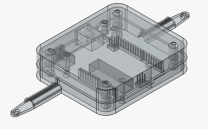
While waiting for the cell to finish cycling, made improvements to the Arduino case on the dev kit:

Looks cleaner and is much easier to assemble, everything can be soldered separately and then installed into the case, rather than trying to solder it while partially in the case.

Stopped the test as the leakage over several days affected things too much. Started hitting the Nernst limit in the final cycles, consistent with loss of active material. On disassembly, there was no zinc, so loss must have come from the iodide, and it was the positive side that was leaking. There was also visible loss of volume. So, didn’t learn too much from this test.

Future tests I will do at higher current to higher SOC to cycle more aggressively.

This test went for 118 hours and 27 cycles, and caues of the leaks, I won’t be comparing it with the previous test. I will do a with/without argon sparging comparison with a tighter setup at higher current/SOC.

Code
import pandas as pd
from tqdm import tqdm, notebook
import numpy as np
import scipy
import plotly.express as px
import plotly.graph_objects as go
from plotly.subplots import make_subplots
import kaleido
from IPython.display import Image

tqdm_disabled = False  # True for website, change to False for local work

sampling = True

MIN_POINTS0 = 500
DIFF_LIMIT = 0.1


# electrolyte component masses, in g
MASS_ZnCl2  = 1.38
MASS_NH4Cl  = 1.06
MASS_KI     = 3.32
MASS_H2O    = 8.50
MASS_TriEG  = 0.55

total_mass_kg = (MASS_ZnCl2 + MASS_KI + MASS_H2O + MASS_TriEG) / 1000.0

TOTAL_VOLUME = 11  # electrolyte volume in mL, approx, measured by taking as much electrolyte as possible up into a 12 mL syringe

MASS_TO_RESERVOIRS = 14.60  # g of electrolyte actually loaded into system, based on weighing syringe before/after loading reservoirs
# molecular weights in g/mol

density = MASS_TO_RESERVOIRS / TOTAL_VOLUME

MW_ZnCl2 = 136.315
MW_NH4Cl = 53.49
MW_KI = 166.0028
MW_H2O = 18.01528
MW_TriEG = 150.174

molality_ZnCl2 = MASS_ZnCl2 / MW_ZnCl2 / total_mass_kg
molality_NH4Cl = MASS_NH4Cl / MW_NH4Cl / total_mass_kg
molality_KI = MASS_KI / MW_KI / total_mass_kg
molality_TriEG = MASS_TriEG / MW_TriEG / total_mass_kg
molality_H2O = MASS_H2O / MW_H2O / total_mass_kg

molarity_ZnCl2 = MASS_ZnCl2 / MW_ZnCl2 / TOTAL_VOLUME * 1000.0
molarity_NH4Cl = MASS_NH4Cl / MW_NH4Cl / TOTAL_VOLUME * 1000.0
molarity_KI = MASS_KI / MW_KI / TOTAL_VOLUME * 1000.0
molarity_TriEG = MASS_TriEG / MW_TriEG / TOTAL_VOLUME * 1000.0
molarity_H2O = MASS_H2O / MW_H2O / TOTAL_VOLUME * 1000.0


filenames = [
    "../lab-notebook-15/16-04-2026-KPS-22.zip",
]


all_data = []
for f in filenames:
    if len(all_data) == 0:
        all_data.append(pd.read_csv(f, delimiter="\t").dropna())
    else:
        df0 = pd.read_csv(f, delimiter="\t").dropna()
        df0["Elapsed time(s)"] += all_data[-1]["Elapsed time(s)"].iat[-1]
        all_data.append(df0)


df = pd.concat(all_data, ignore_index=True)

if not tqdm_disabled:
    print("Electrolyte Composition:")

    print(
        "Molarities (moles/L solution): {:.2f} M ZnCl~2~, {:.2f} M NH~4~Cl, {:.2f} M KI, {:.2f} M triethylene glycol, {:.2f} M H~2~O\n".format(
            molarity_ZnCl2, molarity_NH4Cl, molarity_KI, molarity_TriEG, molarity_H2O
        )
    )
    print(
        "Molalities (moles/kg solution): {:.2f} m ZnCl~2~, {:.2f} m NH~4~Cl, {:.2f} m KI, {:.2f} m triethylene glycol, {:.2f} m H~2~O\n".format(
            molality_ZnCl2, molality_NH4Cl, molality_KI, molality_TriEG, molality_H2O
        )
    )
    print("Density approx. {:.1f} g/mL\n".format(density))
    print(
        "Experiment length: {:.1f} hours".format(
            all_data[-1]["Elapsed time(s)"].iat[-1] / 3600.0
        )
    )


df["mean_current"] = df["Current(A)"].rolling(3).mean()
df["prev_current"] = df["mean_current"].shift(-1)
df["VChange"] = df["Potential(V)"].diff().abs()
df["is_change"] = (
    ((df["mean_current"] > 0) & (df["prev_current"] < 0))
    | ((df["mean_current"] < 0) & (df["prev_current"] > 0))
).astype(int)

idx_changes = list(df[df["is_change"] == 1].index)
idx_changes.append(len(df) - 1)

all_curves = []
idx_start = 0
for idx in tqdm(idx_changes, disable=tqdm_disabled):
    if len(df.iloc[idx_start:idx, :]) > 50:
        all_curves.append(df.iloc[idx_start:idx, :])
    idx_start = idx

results = []
n_curves = np.max([1, int(np.floor(len(all_curves) / 2))])

for CN in notebook.tnrange(n_curves, disable=tqdm_disabled):
    CURVE_N1 = CN * 2
    CURVE_N2 = CN * 2 + 1

    # Process charge data

    if sampling:
        N_TERM_POINTS = int(np.min([MIN_POINTS0, len(all_curves[CURVE_N1]) / 2.0]))
        MIN_POINTS = int(
            np.min([MIN_POINTS0, len(all_curves[CURVE_N1]) - N_TERM_POINTS * 2])
        )

        df0 = pd.concat(
            [
                all_curves[CURVE_N1].iloc[:N_TERM_POINTS],
                all_curves[CURVE_N1]
                .iloc[N_TERM_POINTS:-N_TERM_POINTS]
                .sample(n=MIN_POINTS),
                all_curves[CURVE_N1].iloc[-N_TERM_POINTS:],
            ]
        ).sort_values("Elapsed time(s)", ascending=True)
        df0 = df0[df0["VChange"] < DIFF_LIMIT]
    else:
        df0 = all_curves[CURVE_N1].copy()
    df0["mAh"] = np.abs(
        scipy.integrate.cumulative_trapezoid(
            df0["Current(A)"], df0["Elapsed time(s)"], initial=0
        )
        * 1000.0
        / 3600.0
    )
    total_energy0 = scipy.integrate.cumulative_trapezoid(
        df0["Current(A)"].abs() * df0["Potential(V)"],
        df0["Elapsed time(s)"],
        initial=0.0,
    )[-1]

    # Process discharge data
    if sampling:
        N_TERM_POINTS = int(np.min([MIN_POINTS0, len(all_curves[CURVE_N2]) / 2.0]))
        MIN_POINTS = int(
            np.min([MIN_POINTS0, len(all_curves[CURVE_N2]) - N_TERM_POINTS * 2])
        )
        df1 = pd.concat(
            [
                all_curves[CURVE_N2].iloc[:N_TERM_POINTS],
                all_curves[CURVE_N2]
                .iloc[N_TERM_POINTS:-N_TERM_POINTS]
                .sample(n=MIN_POINTS),
                all_curves[CURVE_N2].iloc[-N_TERM_POINTS:],
            ]
        ).sort_values("Elapsed time(s)", ascending=True)
        df1 = df1[df1["VChange"] < DIFF_LIMIT]
    else:
        df1 = all_curves[CURVE_N2].copy()

    df1["mAh"] = np.abs(
        scipy.integrate.cumulative_trapezoid(
            df1["Current(A)"], df1["Elapsed time(s)"], initial=0.0
        )
        * 1000.0
        / 3600.0
    )
    total_energy1 = scipy.integrate.cumulative_trapezoid(
        df1["Current(A)"].abs() * df1["Potential(V)"],
        df1["Elapsed time(s)"],
        initial=0.0,
    )[-1]

    CE = 100.0 * (df1["mAh"].iloc[-1] / df0["mAh"].iloc[-1])
    EE = 100.0 * (total_energy1 / total_energy0)
    VE = 100.0 * EE / CE
    results.append(
        {
            "Number": CN + 1,
            "CE": CE,
            "VE": VE,
            "EE": EE,
            "Charge_potential": df0["Potential(V)"].mean(),
            "Discharge_potential": df1["Potential(V)"].mean(),
            "Charge_stored": df1["mAh"].iloc[-1] / TOTAL_VOLUME,
            "Energy_density_discharge": total_energy1 / TOTAL_VOLUME / 3600.0 * 1000,
        }
    )

    # Save the modified DataFrames back to the all_curves list
    all_curves[CURVE_N1] = df0
    all_curves[CURVE_N2] = df1

results_df = pd.DataFrame(results)

if not tqdm_disabled:
    print(results_df)
    print("")
    print(results_df.mean())


# Color gradient for charge curves
charge_colors = [
    px.colors.sequential.Blues[int(i)]
    for i in np.linspace(3, len(px.colors.sequential.Blues) - 1, n_curves)
]
discharge_colors = [
    px.colors.sequential.Greys[int(i)]
    for i in np.linspace(3, len(px.colors.sequential.Greys) - 1, n_curves)
]


# Plot charge/discharge curves
fig1 = go.Figure()
for CN in range(n_curves):

    CURVE_N1 = CN * 2
    CURVE_N2 = CN * 2 + 1
    fig1.add_trace(
        go.Scatter(
            x=all_curves[CURVE_N1]["mAh"] / TOTAL_VOLUME,
            y=all_curves[CURVE_N1]["Potential(V)"],
            mode="lines",
            name=f"Charge {CN+1}",
            line=dict(color=charge_colors[CN], dash="solid"),
            showlegend=False,
        )
    )
    fig1.add_trace(
        go.Scatter(
            x=all_curves[CURVE_N2]["mAh"] / TOTAL_VOLUME,
            y=all_curves[CURVE_N2]["Potential(V)"],
            mode="lines",
            name=f"Discharge {CN+1}",
            line=dict(color=discharge_colors[CN], dash="solid"),
            showlegend=False,
        )
    )
fig1.update_layout(
    xaxis_title="Capacity (Ah/L)",
    yaxis_title="Potential (V)",
    legend=dict(orientation="h", yanchor="bottom", y=0.02, xanchor="right", x=0.99),
    hoverlabel=dict(
        bgcolor="white",
    ),
    xaxis=dict(range=[-1, 10]),
    yaxis=dict(range=[-.49, 1.8]),


)

fig1.add_trace(
    go.Scatter(
        x=[None],
        y=[None],
        mode="lines",
        line=dict(color=charge_colors[0], dash="solid"),
        name="Charge (cycle 1)",
    )
)
fig1.add_trace(
    go.Scatter(
        x=[None],
        y=[None],
        mode="lines",
        line=dict(color=charge_colors[-1], dash="solid"),
        name=f"Charge (cycle {n_curves})",
    )
)
fig1.add_trace(
    go.Scatter(
        x=[None],
        y=[None],
        mode="lines",
        line=dict(color=discharge_colors[0], dash="solid"),
        name="Discharge (cycle 1)",
    )
)
fig1.add_trace(
    go.Scatter(
        x=[None],
        y=[None],
        mode="lines",
        line=dict(color=discharge_colors[-1], dash="solid"),
        name=f"Discharge (cycle {n_curves})",
    )
)

fig1.show()
Electrolyte Composition:
Molarities (moles/L solution): 0.92 M ZnCl~2~, 1.80 M NH~4~Cl, 1.82 M KI, 0.33 M triethylene glycol, 42.89 M H~2~O

Molalities (moles/kg solution): 0.74 m ZnCl~2~, 1.44 m NH~4~Cl, 1.45 m KI, 0.27 m triethylene glycol, 34.31 m H~2~O

Density approx. 1.3 g/mL

Experiment length: 118.2 hours

  0%|          | 0/54 [00:00<?, ?it/s]
100%|██████████| 54/54 [00:00<00:00, 5538.39it/s]
    Number         CE         VE         EE  Charge_potential  \
0        1  73.745602  90.687589  66.878109          1.361648   
1        2  76.538573  89.664610  68.628013          1.385708   
2        3  76.930642  90.101953  69.316011          1.234811   
3        4  78.998104  89.789130  70.931711          1.183364   
4        5  79.628673  89.233197  71.055211          1.184038   
5        6  76.038591  90.612553  68.900508          0.963211   
6        7  76.441116  91.158867  69.682856          0.962739   
7        8  78.231445  91.228368  71.369271          0.967186   
8        9  80.667902  90.472015  72.981876          0.972817   
9       10  82.380272  89.900963  74.060658          1.107898   
10      11  79.822890  89.686187  71.590107          1.114498   
11      12  75.103384  91.342760  68.601504          0.967987   
12      13  76.132521  91.376514  69.567244          0.970839   
13      14  78.534972  91.015006  71.478609          0.983610   
14      15  78.744794  90.485612  71.252709          1.162424   
15      16  78.315597  89.996246  70.481097          1.237594   
16      17  73.592674  90.820942  66.837561          1.119237   
17      18  73.936851  91.071991  67.335763          1.073661   
18      19  76.123690  90.649946  69.006083          1.180331   
19      20  78.243235  90.361455  70.701726          1.290355   
20      21  78.577252  89.463758  70.298162          1.344061   
21      22  72.724192  89.774215  65.287572          1.327591   
22      23  69.325215  90.702762  62.879885          1.196238   
23      24  74.534334  90.157728  67.198461          1.215227   
24      25  77.924445  89.879622  70.038197          1.343637   
25      26  76.958185  89.734640  69.058150          1.382980   
26      27  77.836535  89.272540  69.486652          1.391315   

    Discharge_potential  Charge_stored  Energy_density_discharge  
0              0.963598       6.706733                  8.277728  
1              0.842635       6.665409                  8.178791  
2              0.842975       6.995131                  8.599125  
3              0.842687       7.182124                  8.820104  
4              0.842999       7.239415                  8.855880  
5              0.849815       6.912794                  8.545765  
6              0.860636       6.949416                  8.642477  
7              0.858002       7.112091                  8.867715  
8              0.855424       7.333604                  9.108260  
9              0.851634       7.489160                  9.269957  
10             0.859093       7.256904                  8.962803  
11             0.869329       6.827718                  8.550566  
12             0.866772       6.921377                  8.688766  
13             0.871200       7.139648                  8.968549  
14             0.875299       7.158606                  8.990309  
15             0.874370       7.119743                  8.912660  
16             0.887654       6.690454                  8.447672  
17             0.903050       6.721787                  8.519115  
18             0.927451       6.920566                  8.777888  
19             0.951955       7.113026                  9.034405  
20             0.897705       7.143490                  9.014215  
21             0.898535       6.611471                  8.347945  
22             0.907611       6.302529                  8.026840  
23             0.982163       6.762035                  8.639476  
24             0.972786       6.727719                  8.575083  
25             1.000638       6.518383                  8.307315  
26             0.892659       6.249566                  7.925103  

Number                      14.000000
CE                          76.890062
VE                          90.320043
EE                          69.440878
Charge_potential             1.171297
Discharge_potential          0.890692
Charge_stored                6.917441
Energy_density_discharge     8.661278
dtype: float64
(a) Charge/discharge curves
(b)
Figure 1
Code
# Plot efficiency
fig2 = px.scatter(
    results_df,
    x="Number",
    y=["VE", "CE", "EE"],
    labels={"value": "Efficiency (%)", "variable": "Metric"},
)
fig2.update_traces(mode="markers")


fig2.update_layout(
    yaxis=dict(range=[-10, 100]),
    legend=dict(
        orientation="v",
        yanchor="bottom",
        y=0.02,
        xanchor="right",
        x=0.99
    )
)


fig2.show()
Figure 2: Charge/discharge efficiencies
Code
fig5 = px.scatter(
    results_df,
    x="Number",
    y="Energy_density_discharge",
    labels={
        "Energy_density_discharge": "Energy Density on Discharge (Wh/L)",
        "Number": "Cycle Number",
    },
    range_y=[0,1.2*max(results_df["Energy_density_discharge"])]
)

max_val = results_df["Energy_density_discharge"].max()
mean_val = results_df["Energy_density_discharge"].mean()

fig5.add_hline(y=max_val, line_dash="dash", line_color="black", annotation_text="Max", annotation_position="top right",annotation_font_size = 10)
fig5.add_hline(y=mean_val, line_dash="dash", line_color="blue", annotation_text="Mean", annotation_position="top right",annotation_font_size = 10)
fig5.add_hline(y=0.8*max_val, line_dash="dash", line_color="red", annotation_text="80% Max", annotation_position="top right",annotation_font_size = 10)

fig5.show()
Figure 3: Discharge energy densities
Code
norm_charge = results_df["Charge_potential"] / results_df["Charge_potential"].iloc[0]
norm_discharge = results_df["Discharge_potential"] / results_df["Discharge_potential"].iloc[0]

fig6 = go.Figure()
fig6.add_trace(go.Scatter(
    x=results_df["Number"],
    y=norm_charge,
    mode="lines+markers",
    name="Charge Potential"
))
fig6.add_trace(go.Scatter(
    x=results_df["Number"],
    y=norm_discharge,
    mode="lines+markers",
    name="Discharge Potential"
))
fig6.update_layout(
    xaxis_title="Cycle Number",
    yaxis_title="Normalized Potential",
    legend=dict(
        orientation="v",
        yanchor="top",
        y=0.95,
        xanchor="left",
        x=0.05
    )
)

fig6.show()
Figure 4: Average charge and discharge potentials normalized to first cycle
Code
table_df = (
    results_df.describe().loc[["mean", "std"]]
    .round(decimals=1)
    .drop(columns=["Number", "Charge_potential", "Discharge_potential"])
    .rename(
        columns={
            "CE": "Coulombic Efficiency (%)",
            "EE": "Energy Efficiency (%)",
            "VE": "Voltaic Efficiency (%)",
            "Charge_stored": "Discharge Capacity (Ah/L)",
            "Energy_density_discharge": "Energy Density (Wh/L)",
        }
    )
)

# Bar chart of efficiencies with error bars
eff_cols = ["Coulombic Efficiency (%)", "Voltaic Efficiency (%)", "Energy Efficiency (%)"]
eff_labels = ["Coulombic", "Voltaic", "Energy"]

means = table_df.loc["mean", eff_cols].values
stds = table_df.loc["std", eff_cols].values
Code
fig6 = go.Figure()
fig6.add_trace(go.Bar(
    x=eff_labels,
    y=means,
    error_y=dict(type="data", array=stds, visible=True),
    name="Efficiency",
    marker_color=["#1f77b4", "#ff7f0e", "#2ca02c"]
))
fig6.update_layout(
    yaxis_title="Efficiency (%)",
    yaxis=dict(range=[0, 100])
)
fig6.show()
Figure 5: Mean efficiency values with standard deviation
Code
cap_cols = ["Discharge Capacity (Ah/L)"]
cap_labels = ["Discharge Capacity"]

cap_means = table_df.loc["mean", cap_cols].values
cap_stds = table_df.loc["std", cap_cols].values

ed_cols = ["Energy Density (Wh/L)"]
ed_labels = ["Energy Density"]

ed_means = table_df.loc["mean", ed_cols].values
ed_stds = table_df.loc["std", ed_cols].values

fig_combined = make_subplots(rows=1, cols=2)

fig_combined.add_trace(
    go.Bar(
        x=cap_labels,
        y=cap_means,
        error_y=dict(type="data", array=cap_stds, visible=True),
        name="Capacity",
        marker_color="#1f77b4"
    ),
    row=1, col=1
)

fig_combined.add_trace(
    go.Bar(
        x=ed_labels,
        y=ed_means,
        error_y=dict(type="data", array=ed_stds, visible=True),
        name="Energy Density",
        marker_color="#2ca02c"
    ),
    row=1, col=2
)
top = max(max(cap_means + cap_stds), max(ed_means + ed_stds))*1.1
fig_combined.update_layout(
    yaxis=dict(title="Discharge Capacity (Ah/L)"),
    yaxis2=dict(title="Energy Density (Wh/L)", anchor="x2", overlaying="y", side="left"),
    yaxis_range=[0, top],
    yaxis2_range=[0, top],
    showlegend=False
)
fig_combined.show()
Figure 6: Mean discharge capacity and energy density values with standard deviation

Citation

BibTeX citation:
@online{smith2026,
  author = {Smith, Kirk Pollard},
  title = {Lab {Notebook} {Entry} \#16},
  date = {2026-04-22},
  url = {https://dualpower.supply/posts/lab-notebook-16/},
  langid = {en}
}
For attribution, please cite this work as:
K.P. Smith, Lab Notebook Entry #16, (2026). https://dualpower.supply/posts/lab-notebook-16/.